Google Trends API Returns Highly Variable Data
If you are using Google Search data, you should be aware of some basic limitations. Nobody knows the etiology of a search. Searches with the keyword "commit suicide" could be (A) people who are experiencing suicidal ideation, (B) people who want to know if a celebrity committed suicide (e.g., "did Michael Jackson commit suicide"), (C) mental health researchers wondering what comes up when you search "commit suicide", etc.
But that's not all. Google Searches are sampled for each pull, which means that every time they are pulled from the API, they can change. Even when searching the same terms over the same date(s), they can be vastly different. With a simple test, I show the data Google returns is highly variable -- even when you request the same data for the same terms within just a few seconds of each other.
To demonstrate, I pull data for several suicide-related search terms over 10 overlapping time windows.
from gtrendspy import timeline
from datetime import datetime, timedelta
import re
from random import randint
from time import sleep

terms = [
        'commit suicide',
        'suicide statistics',
        'suicide',
        'suicide hotline number',
        'suicide quotes + suicidal quotes',
        'suicide prevention',
        'suicidal thoughts',
        'how to commit suicide',
        'teen suicide',
        'suicide song + suicide songs'
]


## The first date to pull
initial_date = datetime.strptime("2019-03-01", "%Y-%m-%d")

# How different each pull should be
step = 2

# The window for the pull
interval = 360

# Number of pulls
numruns = 10

for index in range(0, numruns):

    # The start date changes with each pull
    start = initial_date + timedelta(days = step * index)
    start_string = start.strftime("%Y-%m-%d")

    # The end date is just the start + interval
    end = start + timedelta(days = interval)
    end_string = end.strftime("%Y-%m-%d")

    # Print the window
    print("start date is {}".format(start_string))
    print("end date is {}".format(end_string))


    # Pull the data
    timeline.theo_timeline(
        terms = terms,
        # I use this to make file names based upon the terms and the run (index)
        names = ["{}_{}".format(re.sub(" \+ | ", "_", x), index) for x in terms],
        start = start_string,
        end = end_string,
        timeframe_list = ['day'],
        geo_country_list = ['US'],
        us_states = False,
        worldwide = False,
        timestep_years = 10,
        batch_size = 5,
        outpath = "~/gtrends-variance/input",
        creds = "~/info_theo.py"
    )

    # I sleep for somewhere between 10 and 20 seconds between each run
    sleep(randint(10,20))
We can then combine this data in R to see whether the different pulls retrieved significantly different values. The first step is to create data frames that merge all the runs for each individual term.
## Arguments
terms <- c(
  'commit suicide',
  'suicide statistics',
  'suicide',
  'suicide hotline number',
  'suicide quotes + suicidal quotes',
  'suicide prevention',
  'suicidal thoughts',
  'how to commit suicide',
  'teen suicide',
  'suicide song + suicide songs'
)

timeframe <- 'day'
ROOTPATH <- "~/gtrends-variance"


## Load packages
if(!require("pacman")) install.packages("pacman")
pacman::p_load(dplyr, tidyverse, gsubfn, psych, lubridate, reshape2)


## Build Data

# Get all the file names for that term
setwd(ROOTPATH)
files <- dir("./input", ".csv", full.name = T)
files <- grep(timeframe, files, value = T)
names <- gsub(" [+] | ", "_", terms)


# Create empty lists to fill in through a for loop
summ_data_list <- list()
full_data_list <- list()
ct <- 1

# For each term
for(name in names){

  # We take all the files with that term
  same_files <- grep(name, files, value = T)
  # ... read them in and merge them into a list
  dat <- list()
  for(f in same_files){
    term <- basename(f)
    num <- strapplyc(term, "_([0-9]+)_[A-Za-z]+.csv$") %>% as.numeric() + 1
    df <- read.csv(f, header = T, stringsAsFactor = F)
    names(df) <- c("timestamp", paste0("run", num))
    dat[[num]] <- df
  }

  # Which we then combine
  df <- Reduce(function(x, y) merge(x, y, by="timestamp", all = F), dat)

  # We only use those dates where there was no missing values across pulls
  df <- df %>% filter(complete.cases(df))


  # We can get some summary statistics on the rows

  # `tmp' allows us to use the rows without worrying about timestamp`
  tmp <- df %>% select(-timestamp)
  summ_data <- data.frame(
    timestamp = ymd(df$timestamp),
    # we get the sd by row
    sd = apply(tmp, 1, function(x) sd(x)),
    # the mean by row
    mean = apply(tmp, 1, function(x) mean(x)),
    # the min by row
    min = apply(tmp, 1, function(x) min(x)),
    # the max by row
    max = apply(tmp, 1, function(x) max(x))
    ) %>% mutate(
    # compute a few interesting numbers
    sd_over_mean = sd / mean,
    range = max - min,
    range_over_mean = range / mean
  )

  # We add these to lists of data
  summ_data_list[[ct]] <- summ_data
  names(summ_data_list)[ct] <- name
  full_data_list[[ct]] <- df
  names(full_data_list)[ct] <- name
  ct <- ct + 1

}
Each data frame in full_data_list corresponds to the raw data for a different term by timestamp. I am unable to share this data because it is raw data, but the first column is timestamp, the second is run1, then run2, up to run10. Under each run column is the search volume for the date. If you run this code on your own, you will see that the search values are different among runs -- even though are for the same query on the same date using the same API executed just seconds apart.
Each data frame in summ_data_list corresponds to a summary of a different term by timestamp. The rows are different dates, and there are statistics related to the variance of the rows in the columns. Here is the raw data table for the search term commit suicide.
| timestamp | sd | mean | min | max | sd_over_mean | range | range_over_mean |
|---|---|---|---|---|---|---|---|
| 2019-03-19 | 6.318569 | 16.39029 | 9.341083 | 31.61500 | 0.3855068 | 22.27392 | 1.3589704 |
| 2019-03-20 | 6.097820 | 20.33431 | 9.597624 | 32.24064 | 0.2998784 | 22.64302 | 1.1135375 |
| 2019-03-21 | 4.726079 | 11.74259 | 6.313096 | 18.91806 | 0.4024734 | 12.60496 | 1.0734399 |
| 2019-03-22 | 4.210195 | 16.64089 | 12.957275 | 26.11812 | 0.2530030 | 13.16085 | 0.7908740 |
| 2019-03-23 | 4.667966 | 10.13054 | 7.442979 | 18.78849 | 0.4607815 | 11.34551 | 1.1199317 |
| 2019-03-24 | 5.416404 | 27.51927 | 21.182260 | 38.60976 | 0.1968222 | 17.42750 | 0.6332837 |
We can summarize these date-level statistics to get a better sense for how much variance we can expect for the average observation. For example, it appears that the range between the highest and lowest observation on any given date is typically a meaningful percentage of the query fraction.
lapply(summ_data_list, function(x) sprintf("%.2f%%", mean(x$range_over_mean) * 100)) %>%
  data.frame() %>% t() %>% kable(format = "markdown")
| commit_suicide | 101.47% |
| suicide_statistics | 97.15% |
| suicide | 87.14% |
| suicide_hotline_number | 105.60% |
| suicide_quotes_suicidal_quotes | 92.52% |
| suicide_prevention | 50.12% |
| suicidal_thoughts | 65.09% |
| how_to_commit_suicide | 101.47% |
| teen_suicide | 87.14% |
| suicide_song_suicide_songs | 77.63% |
This means, for example, the range in search volumes over 10 API runs for the keyword "commit suicide" is, on average, 101% of its mean. That is, if you were to request this data 10 different times for the same date, you would expect that the maximum value you got would be more than twice the minimum value you got. In fact, we can see how large this range could be:
lapply(summ_data_list, function(x) sprintf("%.2f%%", max(x$range_over_mean) * 100)) %>%
  data.frame() %>% t() %>% kable(format = "markdown")
| commit_suicide | 230.46% |
| suicide_statistics | 205.66% |
| suicide | 236.32% |
| suicide_hotline_number | 213.62% |
| suicide_quotes_suicidal_quotes | 213.75% |
| suicide_prevention | 130.47% |
| suicidal_thoughts | 128.33% |
| how_to_commit_suicide | 230.46% |
| teen_suicide | 236.32% |
| suicide_song_suicide_songs | 190.79% |
This means that the range between the minimum and maximum value you got could be as high as 230% of the mean!
You can also see the size of the average range between minimum and maximum values for each time point.
lapply(summ_data_list, function(x) sprintf("%.2f", mean(x$range))) %>%
  data.frame() %>% t() %>% kable(format = "markdown")
| commit_suicide | 17.02 |
| suicide_statistics | 20.35 |
| suicide | 24.46 |
| suicide_hotline_number | 16.20 |
| suicide_quotes_suicidal_quotes | 22.35 |
| suicide_prevention | 39.25 |
| suicidal_thoughts | 30.95 |
| how_to_commit_suicide | 17.02 |
| teen_suicide | 24.46 |
| suicide_song_suicide_songs | 25.11 |
This means that, if you chose the run with the highest search volume for any particular date, you'd expect to be able to say "suicide statistics" was 20.35 (searches per 10M) higher than if you were to choose the run with the lowest search volume. We can also see how large this range can be:
lapply(summ_data_list, function(x) sprintf("%.2f", max(x$range))) %>%
  data.frame() %>% t() %>% kable(format = "markdown")
| commit_suicide | 39.08 |
| suicide_statistics | 42.42 |
| suicide | 57.37 |
| suicide_hotline_number | 39.76 |
| suicide_quotes_suicidal_quotes | 46.24 |
| suicide_prevention | 117.79 |
| suicidal_thoughts | 61.67 |
| how_to_commit_suicide | 39.08 |
| teen_suicide | 57.37 |
| suicide_song_suicide_songs | 61.05 |
This means that for one date, the difference between the highest and lowest pull for searches with the query "suicide prevention" was 118 searches per 10M. Given that this is daily data, that is a difference of approximately 11,000 searches in a single day!
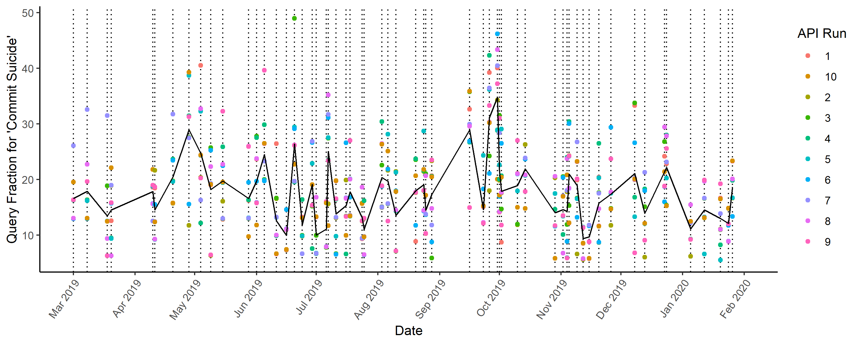
We can visualize how different individual runs are from the mean with a dot plot. We use searches for "commit suicide" as an example. Each vertical line is a (randomly sampled) date. The black line is the mean for all runs, and the colored dots represent a different run.
set.seed(1234)
df <- full_data_list[[1]]
long_df <- melt(df %>% filter(complete.cases(.)) %>% sample_n(60), id = "timestamp", value.name = "searches", variable.name = "run")
long_df$run <- gsub("run", "", long_df$run)
long_df$timestamp <- ymd(long_df$timestamp)
long_df <- long_df %>% arrange(timestamp)

grouped_df <- long_df %>% group_by(timestamp) %>% summarise(meansearches = mean(searches, na.rm = T)) %>% ungroup()

p <- ggplot(long_df)
p <- p + geom_vline(aes(xintercept = timestamp), linetype = "dotted")
p <- p + geom_point(aes(x = timestamp, y = searches, col = run))
s1 <- seq.Date(min(ymd(long_df$timestamp)), max(ymd(long_df$timestamp)) + 28, by = "1 month")
p <- p + scale_x_date(
    lim = c(min(s1), max(s1)),
    breaks = s1,
    labels = function(x) format(x, format = "%b %Y")
  )
p <- p + geom_line(data = grouped_df, aes(x=timestamp, y = meansearches))
p <- p + theme_classic()
p <- p + theme(axis.text.x = element_text(angle = 55, hjust = 1))
p <- p + labs(
  x = "Date",
  y = "Query Fraction for 'Commit Suicide'",
  col = "API Run"
)

ggsave("./output/commitsuicide_dotplot.png", p, width = 10, height = 4)
In summary, when you request the search volume for a given term on a given date from the Google Trends API, you need to know that this data is sampled. From this basic test, it seems that the data Google returns is, in itself, highly variable -- even when you request the same data for the same terms within just a few seconds of each other. Standard statistical analyses that assume each data point is its true value (rather than a value with randomness of its own) will underestimate standard errors.